Decision Models in Practice: When Picking the LLM per Message Pays Off (and When the Mid-Tier Model Is Enough)
“I only returned the backpack from order 10407, which had a coupon, and the refund came in lower. I want the math.”
Looks like any other refund question. It isn’t. Order 10407 has no coupon at all. The customer is wrong, and the model has to notice that before it starts doing arithmetic.
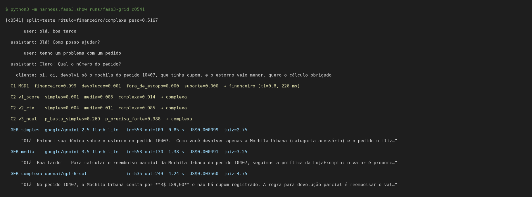
I sent that message (in Portuguese, the chatbot’s language) to the three models in my test chatbot. The cheapest one scored 2.75 from the judge. The mid-tier one, 3.25. Only the expensive one noticed there was no coupon, and it scored 4.75.
That’s the whole problem in one example. Most post-sales messages are “where’s my order?”, and any model handles them. But every now and then one of these shows up. Send everything to the expensive model and you pay premium prices to answer tracking questions. Send everything to the cheap one and you botch the backpack.
This post is about a POC I built to measure exactly that: a post-sales chatbot where a decision model, Microsoft-Decision-1, picks the subagent and the LLM for each message. I’ll walk through the harness, the real payloads, the code that matters, how I calibrated the threshold, how the stats work, and what changed between a small run and a big one.
Everything is in the public repo: github.com/gabrielcaiana/poc-modelos-de-decisao. The code comments and labels are in Portuguese; I translate the bits that matter as we go.
Table of contents
- The bottom line first
- The design: three subagents, two decisions
- What a call to MSD1 looks like
- Layer 1: routing with a threshold
- Layer 2: three ways to ask “is this one hard?”
- The harness: collect the grid, apply the policy later
- The cost guard
- How the dataset was generated
- The statistics, demystified
- Run 1: the decision model seemed to lose
- Run 2: 1,000 conversations
- Where MSD1 wins, and why that’s exploratory
- The bottleneck is spotting the hard case
- What I can’t claim
- How to reproduce it
- What’s next
The bottom line first
If you’re in a hurry:
- Routing with a decision model works. MSD1 got 94.1% of clear messages right on the test set, with calibrated probabilities and ~230 ms per decision.
- Against the expensive model, per-message model selection matches quality at 77% to 82% lower cost.
- Against the mid-tier model, I can’t claim an advantage. There’s a difference (+0.041 on the score), but it isn’t statistically significant.
- The difference shows up on hard cases, but I decided to look there after seeing the data, so it’s a hypothesis, not a result.
Picking the model per message only pays off when you can reliably spot the hard case. Most of the time, the mid-tier model is enough.
The design: three subagents, two decisions
The chatbot handles post-sales for “LojaExemplo”, a made-up store with 60 fake orders. The tools (order lookup and store policy) are deterministic mocks, and their output goes into the subagent’s prompt.
There are three subagents:
| Subagent | Handles |
|---|---|
devolucao (returns) | returns, exchanges, change of mind, defects, return labels and pickup |
suporte (support) | tracking, delivery, address, pre-shipment cancellation, account, product usage |
financeiro (billing) | refunds, charges, chargebacks |
Before generating a single word, two decisions happen:
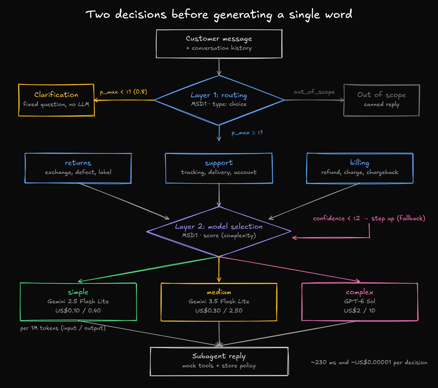
The two decisions: routing with a threshold and model selection across three tiers.
The three models form a real price ladder (USD per 1M tokens, OpenRouter, Oct 12, 2026):
| Tier | Model | Input | Output | max_tokens |
|---|---|---|---|---|
| simple | google/gemini-2.5-flash-lite | 0.10 | 0.40 | 400 |
| medium | google/gemini-3.5-flash-lite | 0.30 | 2.50 | 400 |
| complex | openai/gpt-6-sol | 2.00 | 10.00 | 800 |
GPT-6 Sol gets a higher max_tokens because reasoning tokens count as output. No response was truncated on any model.
One trade-off I accepted: cheap and mid-tier come from the same family. The price ladder is clean, but the mid-tier model is strong enough to be hard to beat.
What a call to MSD1 looks like
Microsoft-Decision-1 (microsoft/microsoft-decision-1, version -20261009) doesn’t generate text. You send a state and one or more questions with fixed options, and it returns a probability for each option. I used OpenRouter’s decisions endpoint, POST https://openrouter.ai/api/alpha/decisions.
The harness client is plain stdlib:
# harness/client.py
def decide(self, model, state, questions):
    p = self.prices.get(model, {"in": 0.042e-6, "out": 0})
    reserve = (est_tokens(json.dumps(state, ensure_ascii=False) + json.dumps(questions, ensure_ascii=False)) + 400) * max(p["in"], 1e-7) * 2
    self.budget.check(reserve)
    t0 = time.perf_counter()
    r = self._post("/alpha/decisions", {"model": model, "state": state, "questions": questions})
    lat = (time.perf_counter() - t0) * 1000
    cost, src = self._cost(model, r.get("usage", {}), "input_tokens", "output_tokens")
    self.budget.add(model, cost)
    ...
Here’s the actual Layer 1 request body for the opening message (conversation c0541), rebuilt by the code itself from the dataset. I left it in the original Portuguese:
{
  "model": "microsoft/microsoft-decision-1",
  "state": {
    "historico": [
      {"role": "user", "content": "olá, boa tarde"},
      {"role": "assistant", "content": "Olá! Como posso ajudar?"},
      {"role": "user", "content": "tenho um problema com um pedido"},
      {"role": "assistant", "content": "Claro! Qual o número do pedido?"}
    ],
    "mensagem_cliente": "oi, oi, devolvi só o mochila do pedido 10407, que tinha cupom, e o estorno veio menor. quero o cálculo obrigado"
  },
  "questions": {
    "subagente": {
      "type": "choice",
      "instructions": "Qual subagente do atendimento pós-venda deve tratar a última mensagem do cliente?",
      "criteria": {
        "devolucao": "Devolução, troca, arrependimento, produto com defeito/errado que o cliente quer devolver ou trocar, etiqueta e coleta de devolução.",
        "suporte": "Status e rastreio de pedido, entrega/atraso/extravio, endereço, cancelamento antes do envio, conta/cadastro, uso e configuração de produto.",
        "financeiro": "Reembolso, cobrança (duplicada, indevida, juros, boleto), estorno no cartão ou Pix, valores pagos e devolvidos.",
        "fora_de_escopo": "Assunto não relacionado a pedidos, produtos ou pagamentos da loja."
      }
    }
  }
}
Notice that each option’s description is the prompt. That’s where you tune routing, not in the system prompt of a generative LLM.
The harness doesn’t keep the raw HTTP response. It keeps what matters, one record per decision, in runs/fase3-grid/grid.jsonl. For the same conversation:
{"id": "c0541", "tipo": "c1",
 "probs": {"devolucao": 0.000626, "financeiro": 0.999271, "fora_de_escopo": 0.0000514, "suporte": 0.0000514},
 "raw_choice": "financeiro", "p_max": 0.999271,
 "cost": 1.1088e-05, "lat_ms": 226.1, "model": "microsoft/microsoft-decision-1-20261009"}
(Probabilities rounded to fit; the file has full precision.)
A decision like this costs around US$0.00001. MSD1 charges US$0.042 per million input tokens, and output is basically nothing: the usage records show 1 or 2 output tokens.
Layer 1: routing with a threshold
Layer 1 is short:
# harness/pipeline.py
def camada1(client, state, tau1=None):
    tau1 = TH["tau1"] if tau1 is None else tau1
    d = client.decide(MODELS["msd1"], state, {"subagente": Q_SUBAGENTE})
    a = d["answers"]["subagente"]
    pmax = max(a["probabilities"].values())
    choice = a["choice"] if pmax >= tau1 else "clarificar"
    ...
If the top probability is below τ1, the chatbot doesn’t guess. It sends a fixed question, no LLM involved: “is this about a return/exchange, your order/delivery, or a refund/charge?”. The only cost is the decision.
This only works if the probabilities are honest, meaning that when the model says 0.95 it’s right about 95% of the time. That’s calibration. In the first run, the ECE (the average gap between stated confidence and actual accuracy) was 0.054.
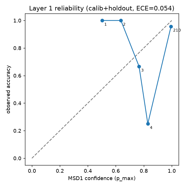
How τ1 was calibrated
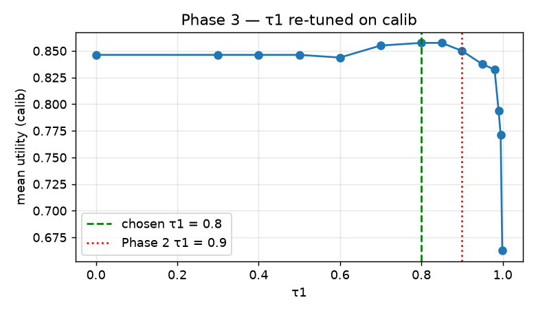
I didn’t eyeball the threshold. I defined a utility function before looking at the test set and swept a grid of values on the calibration split:
# harness/fase3/replay.py (same utility as harness/calibrate.py)
def u1(c, it, tau):
    """+1 right; +1 clarified an ambiguous one; +0.5 ambiguous routed to an accepted label; -1 wrong; 0 clarified a clear one"""
    acc = c["p_max"] >= tau; ch = c["raw_choice"]; lab = it["label"]
    if lab == "clarificar": return 1 if not acc else (0.5 if ch in (it.get("aceitos") or []) else -1)
    return (1 if ch == lab else -1) if acc else 0
In plain terms: a correct route is +1, a wrong one is −1, asking when the message was clear is 0 (it costs the customer a turn but breaks nothing), and asking when the message was genuinely ambiguous is +1.
In phase 3, the calibration curve looked like this:
| τ1 | 0.0–0.5 | 0.7 | 0.8 | 0.85 | 0.9 | 0.95 | 0.99 | 0.999 |
|---|---|---|---|---|---|---|---|---|
| utility | 0.846 | 0.855 | 0.858 | 0.858 | 0.850 | 0.838 | 0.794 | 0.663 |
0.8 and 0.85 tied. Ties go to the lower τ (fewer clarifications), so it landed on τ1 = 0.8. That value was written to config/fase3_congelado.json at 09:54 on Oct 12, 2026 (São Paulo time), before any test metric was computed.
On the test set, the trade-off is right there in the numbers:
| τ1 | Clarification | Error among accepted | Ambiguous handled well | Utility |
|---|---|---|---|---|
| 0.9 (run 1) | 5.2% | 4.6% | 89.5% | 0.848 |
| 0.8 (recalibrated) | 2.8% | 4.7% | 81.6% | 0.848 |
| no threshold | 0.0% | 5.9% | 81.6% | 0.841 |
At 0.8 the chatbot asks less often but handles ambiguous messages worse. On utility, it’s a tie. A high threshold means more questions for the customer; a low one means more silent mistakes. With calibrated probabilities, that trade-off becomes a number you choose instead of a guess.
Layer 2: three ways to ask “is this one hard?”
Layer 2 picks the model tier. In run 1 it was a single score question from 0 to 2. In phase 3 I tested three variants, all in harness/fase3/variantes.py:
v1_score: the original question, with no order data in thestate.v2_ctx: still a 0–2 score, but the tool output goes into thestateand the criteria focus on cross-checking order data against policy.v3_noul: two yes/no questions in a single call: “is the small model enough?” and “does this need the strong model?”.
v2_ctx came out of a finding from run 1 (I’ll get there). Its criteria, roughly translated: simple means you can answer from policy alone or one direct order field; medium means you must cross order data (status, days since delivery, items, category, payment) with policy; complex means multiple issues, a policy exception, value calculations with coupons or partial returns, a mismatch between what the customer says and the data, fraud, or an angry customer.
Q_V2 = {"type": "score", "instructions": "Qual o nível mínimo de modelo para responder CORRETAMENTE esta mensagem, considerando os dados do pedido e a política?",
        "criteria": [
            "simples: dá para responder só com a política ou com um dado direto do pedido, sem cruzar informações nem tirar conclusões",
            "media: é preciso cruzar dados do pedido (status, dias desde a entrega, itens, categoria, pagamento) com a política para decidir o que vale",
            "complexa: vários problemas, exceção de política, cálculo de valores com cupom/parcial, divergência entre o que o cliente diz e os dados, fraude ou cliente irritado"]}
The state gets the tool output. For c0541:
[ferramenta status_pedido(10407)] -> {'pedido': '10407', 'status': 'em_transito', ..., 'itens': [{'nome': 'Kit Panelas 5pç', ...}, {'nome': 'Mochila Urbana', 'preco': 189.0, 'categoria': 'acessorio'}, ...], 'cupom': None, 'total_pago': 667.9, 'cobrancas': 1}
The decision policy lives apart from the call. Each variant returns raw probabilities, and the threshold is applied afterwards:
def politica(rec, variante, params):
    p = rec["probs"]
    if variante in ("v1_score", "v2_ctx"):
        raw = max(ORD, key=lambda t: p[t])
        if p[raw] >= params["tau"]: return raw
        return "complexa" if params.get("fallback", "complexa") == "complexa" else ORD[min(ORD.index(raw) + 1, 2)]
    if p["p_basta_simples"] >= params["ta"]: return "simples"
    return "complexa" if p["p_precisa_forte"] >= params["tb"] else "media"
For c0541, all three variants agreed: v1_score gave complex 0.914, v2_ctx gave 0.985, and v3_noul gave “needs the strong model” 0.988. They sent it to GPT-6 Sol, the only model that got it right.
The harness: collect the grid, apply the policy later
The most important design decision in the harness was this: don’t run each strategy separately.
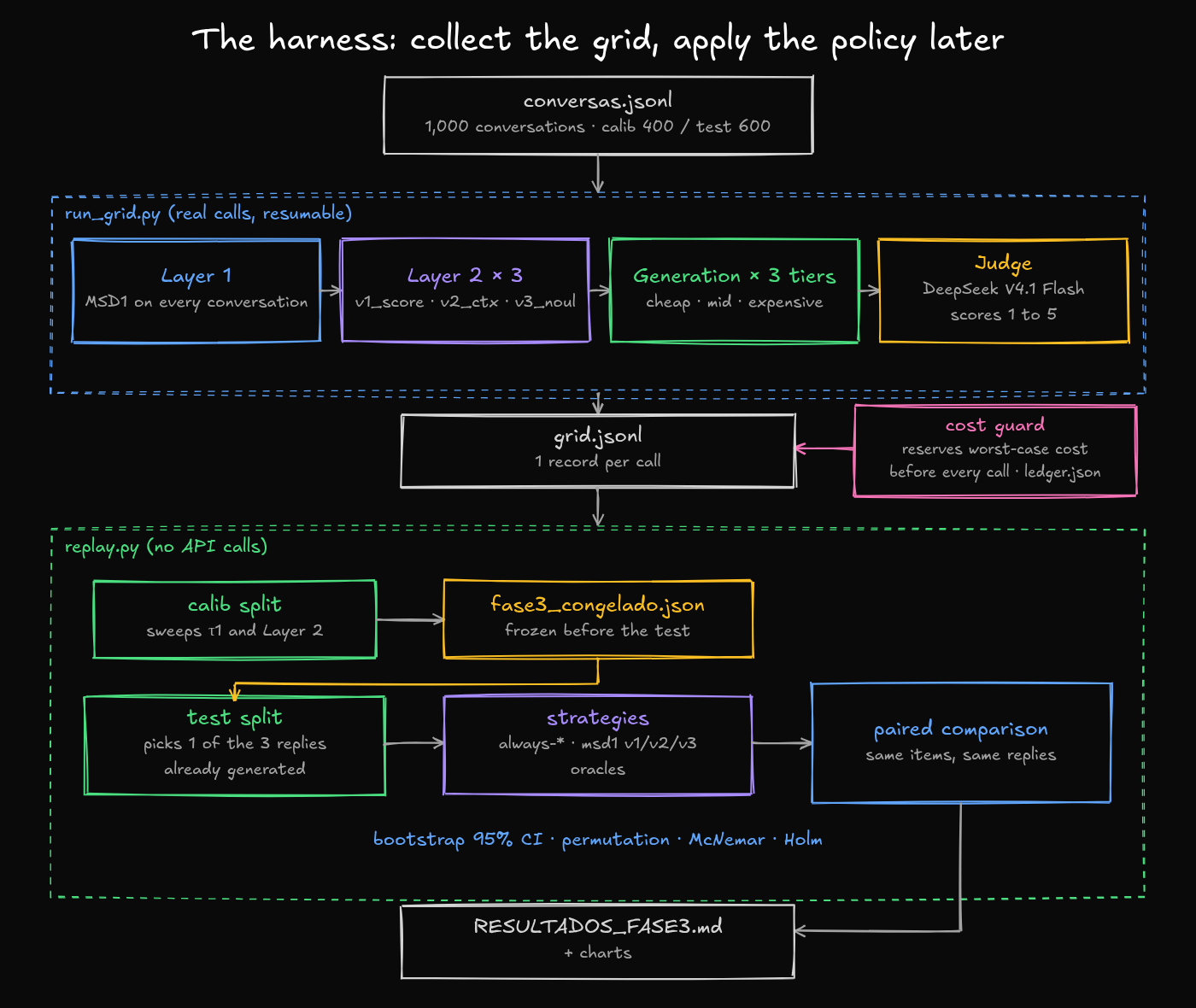
The grid records every call once; replay evaluates every strategy without calling the API.
harness/fase3/run_grid.py does a grid collection. For each conversation it:
- runs Layer 1;
- for routed messages, runs all three Layer 2 variants (decisions only, cheap);
- for items flagged for generation, generates the reply with all three models and calls the judge on each one.
Everything goes into grid.jsonl, one record per call. Then harness/fase3/replay.py evaluates any strategy (always-cheap, always-mid, always-expensive, MSD1 with any variant and threshold, the oracles) without calling the API again. For each item, it just picks which of the three already-generated replies that strategy would have used.
Two wins:
- Perfect pairing. Every strategy is compared on the same messages with the same replies. The only difference between them is the model choice.
- Threshold sweeps are free. The Layer 2 grid has 18 combinations for
v1/v2and 49 forv3, and none of them costs an extra call.
The grid is also resumable: if it dies halfway, it reads what’s done and carries on.
The judge is deepseek/deepseek-v4.1-flash, from a different model family, at temperature 0 with JSON output. It scores correctness, resolution, policy and tone from 1 to 5. A reply “passes” if the average is ≥ 4.5 and the policy score is ≥ 4.
The cost guard
Running 1,000 conversations across three models with a judge per reply shouldn’t be an act of faith. The guard lives in harness/budget.py, and the rule is simple: before every call, reserve the worst-case cost.
# harness/budget.py
def check(self, reserve_usd: float):
    if self.spent + reserve_usd > self.stop_at:
        raise BudgetExceeded(f"gasto acumulado US${self.spent:.4f} + reserva US${reserve_usd:.4f} > parada US${self.stop_at}")
    if self.session_cap is not None and self.session_spent + reserve_usd > self.session_cap:
        raise BudgetExceeded(...)
For chat calls, the reservation is estimated prompt tokens × input price + max_tokens × output price, plus a 20% buffer. After the call, the real cost (the usage.cost OpenRouter returns) goes into a persistent ledger, runs/ledger.json.
The setup: a hard cap of US$20 with an automatic stop at US$18 (config/budget.json), an optional per-run --session-cap, and the same US$20 limit configured on the OpenRouter key itself. At the end I reconciled the ledger against GET /api/v1/key.
The whole POC cost US$1.66. Phase 3 alone was US$1.35.
How the dataset was generated
The phase 3 dataset comes from datasets/fase3/gerar_conversas.py: deterministic combinatorial templates with a fixed seed, written with help from an LLM. Labels are derived by rule from explicit attributes of each scenario.
The complexity rule:
- simple: a policy/FAQ question or a direct lookup, no cross-checking order data against policy;
- medium: requires crossing order data (status, days, items, payment) with policy, one issue;
- complex: 2+ issues, a policy exception, a value calculation (coupon/partial), fraud/risk, or an angry customer with a history of failures.
Each conversation has 0 to 3 prior turns (greeting, the bot asking for the order number, the customer giving it) and a final message, which is the one being evaluated. Sometimes the order number only appears in the history. On top of that, the generator adds noise: prefixes, suffixes (“pls”, ”??”, “it’s urgent”), texting abbreviations, and typos like “pedio” for “pedido”.
The mix: 1,000 conversations, 4% out of scope and 6% ambiguous. Among routable messages, complexity targets roughly 60/28/12 (simple/medium/complex). The split is 400 for calibration and 600 for test, with no exact duplicates across them.
Generating replies with all three models for everything would be expensive and pointless. So generation runs on a stratified subset, 150 items in calibration and 300 in test, oversampling the complex tail to get statistical power on the hard cases. Each item carries a peso (weight) that undoes the oversampling, so every average is weighted back to the realistic mix. After removing what Layer 1 clarified or flagged as out of scope, that leaves 140 evaluable items in calibration and 265 in test.
An honest caveat on “multi-turn”: the history is real and gets passed to MSD1 and to the subagent, but it’s scripted. The chatbot decides and replies once, on the last message. It’s not a full conversation running end to end.
The statistics, demystified
When MSD1 scores 4.629 and the mid-tier model scores 4.588, the real question is: if I ran this on different conversations, would that gap still be there?
replay.py answers with four tools, all paired (same items, item-by-item differences):
- Bootstrap (95% CI). Resample the 265 items with replacement 5,000 times and recompute the weighted mean difference each time. The range between the 2.5th and 97.5th percentiles is the 95% CI: where the true difference most likely sits. If it includes zero, “no difference” is still on the table.
- Permutation test (sign flip). If the two strategies were equivalent, it wouldn’t matter whether an item’s difference is +0.25 or −0.25. So I flip each difference’s sign at random, 5,000 times, and count how often the result is as extreme as what I observed. That fraction is the p-value.
- McNemar. For pass/fail, only the items where the strategies disagree matter: one passes, the other doesn’t. If they were equivalent, those disagreements should split roughly 50/50. McNemar checks that with an exact binomial.
- Holm correction. I ran 6 comparisons (3 variants × 2 baselines). The more tests you run, the likelier one comes up “significant” by luck. Holm sorts the p-values and multiplies each by a shrinking factor (6, 5, 4…), raising the bar to compensate.
McNemar and Holm fit in a few lines:
b01 = sum(1 for x, y in zip(a["_p"], b["_p"]) if x and not y)
b10 = sum(1 for x, y in zip(a["_p"], b["_p"]) if y and not x)
mcn = 1.0 if b01 + b10 == 0 else min(1.0, 2 * sum(math.comb(b01 + b10, k) for k in range(0, min(b01, b10) + 1)) / 2 ** (b01 + b10))

def holm(ps):
    ordem = sorted(range(len(ps)), key=lambda i: ps[i]); adj = [0] * len(ps); m = len(ps); run = 0
    for k, i in enumerate(ordem): run = max(run, min(1, (m - k) * ps[i])); adj[i] = run
    return adj
The most important part isn’t statistical, though. It’s process: the tuning rule was written down first. Among the parameters whose calibration score is within 0.05 of always-mid, pick the cheapest. The chosen parameters were frozen before looking at the test set, and replay.py has an assert that fails if a recomputed tuning disagrees with the frozen one.
Run 1: the decision model seemed to lose
Before phase 3 there was a small run: 300 single-turn messages, 60 of them in the test set.
| Strategy | Savings vs always-expensive | Judge score |
|---|---|---|
| always-expensive | 0% | 4.71 |
| always-mid | 83.7% | 4.60 |
| MSD1 | 78.3% | 4.48 |
| always-cheap | 96.7% | 4.18 |
Always-mid was cheaper and scored higher. The obvious conclusion would have been “Layer 2 doesn’t pay for itself.”
But with 60 messages, score differences under ~0.3 weren’t conclusive. I had a signal, not an answer. So I designed phase 3 before calling it.
Run 2: 1,000 conversations
On the phase 3 test set (265 items, weighted averages):
| Strategy | Score | % pass | US$/msg | Latency P50 / P95 |
|---|---|---|---|---|
| always-expensive (GPT-6 Sol) | 4.652 | 89.2% | 0.002238 | 3.50 s / 5.63 s |
MSD1 v2_ctx | 4.629 | 88.7% | 0.000512 | 1.47 s / 4.98 s |
MSD1 v1_score | 4.614 | 88.5% | 0.000427 | 1.40 s / 5.04 s |
MSD1 v3_noul | 4.605 | 87.2% | 0.000401 | 1.41 s / 4.82 s |
| always-mid | 4.588 | 85.9% | 0.000335 | 1.33 s / 1.92 s |
| always-cheap | 4.457 | 79.8% | 0.000072 | 0.94 s / 1.77 s |
| empirical oracle | 4.706 | 96.7% | 0.000345 | 1.02 s / 4.47 s |
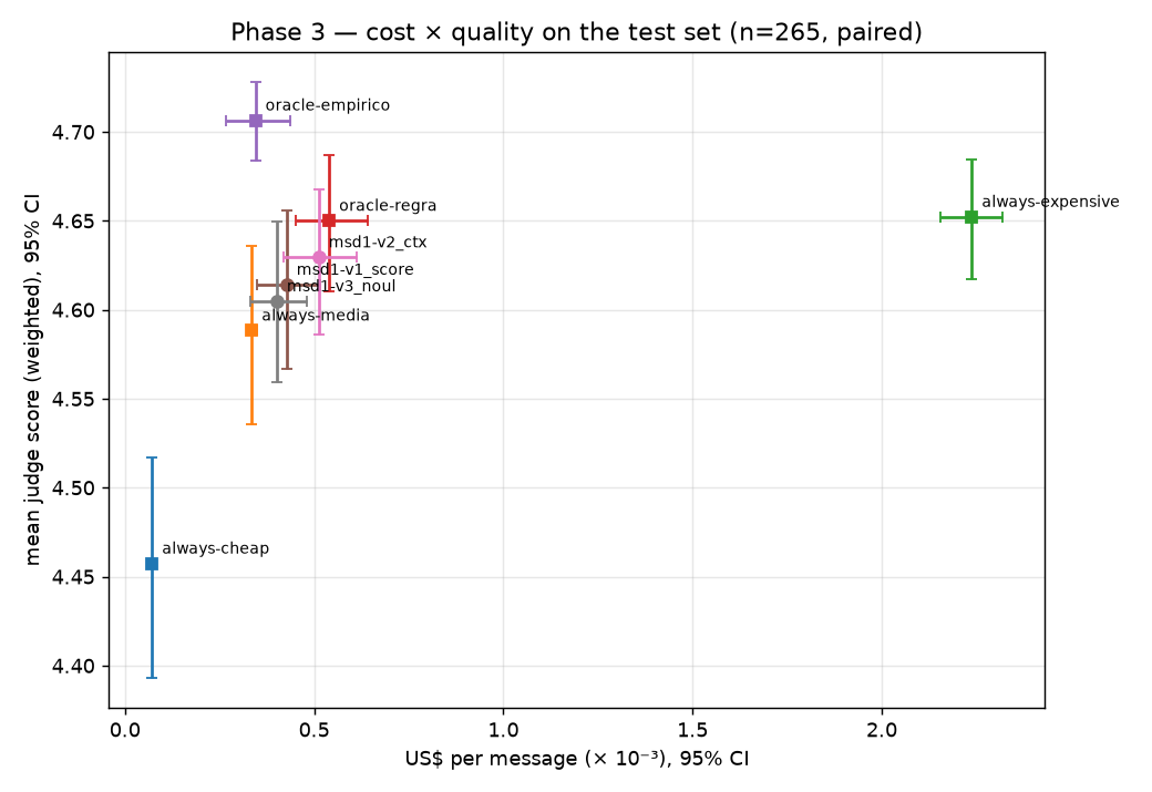
The paired comparisons:
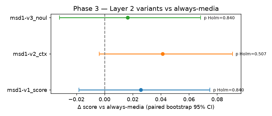
| Comparison | Δ score (95% CI) | Holm p | McNemar Holm p |
|---|---|---|---|
v2_ctx vs always-mid | +0.041 (−0.004; +0.091) | 0.51 | 0.054 |
v1_score vs always-mid | +0.026 (−0.018; +0.075) | 0.84 | 0.057 |
v3_noul vs always-mid | +0.016 (−0.032; +0.068) | 0.84 | 0.43 |
v2_ctx vs always-expensive | −0.023 (−0.074; +0.028) | 0.84 | 0.92 |
v1_score vs always-expensive | −0.038 (−0.091; +0.013) | 0.63 | 0.92 |
v3_noul vs always-expensive | −0.047 (−0.102; +0.005) | 0.51 | 0.46 |
What that means:
- Against always-mid, every CI includes zero and no p-value gets under 0.05. The McNemar for
v2_ctxcomes close (0.054): it passed 25 items where always-mid failed, versus 9 the other way. Close, but no. MSD1 looks slightly better, and I can’t claim it is. - Against always-expensive, nothing significant either, but the reading flips: statistically equal quality at 77% to 82% lower cost, depending on the variant.
Also look at P95 latency: always-mid sits at 1.92 s, while every MSD1 variant is close to 5 s. That’s not the decision overhead (~0.2–0.5 s). That’s GPT-6 Sol showing up in the tail.
Where MSD1 wins, and why that’s exploratory
Breaking the score down by the rule’s complexity tier:
| Strategy | simple | medium | complex |
|---|---|---|---|
| always-cheap | 4.64 | 4.45 | 3.56 |
| always-mid | 4.64 | 4.66 | 4.15 |
| always-expensive | 4.62 | 4.70 | 4.66 |
MSD1 v2_ctx | 4.64 | 4.63 | 4.57 |
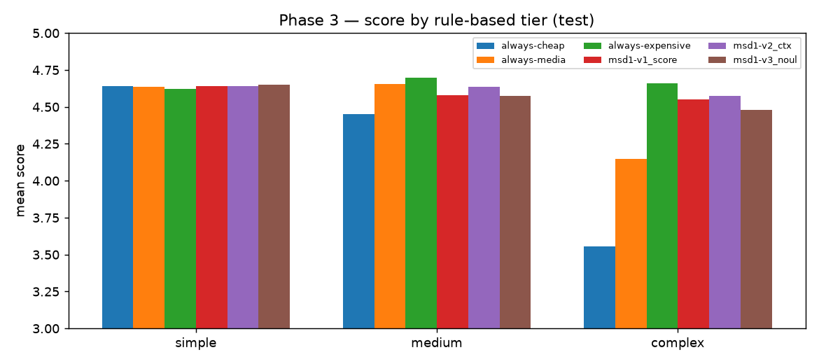
On simple cases everyone ties, the cheap model included. On complex ones, always-mid drops to 4.15.
Across the 57 complex cases in the test set, MSD1 lands about +0.4 above always-mid: v2_ctx +0.425 (95% CI +0.27 to +0.59), v1_score +0.404, v3_noul +0.329.
Big asterisk. This analysis is post hoc: I decided to slice by complexity after seeing the per-tier breakdown. It wasn’t in the plan, and I didn’t apply any extra correction. It’s good for generating the next hypothesis, not for proving anything.
The bottleneck is spotting the hard case
The empirical oracle is a “cheating” strategy: for each item, it uses the cheapest model whose score is within 0.25 of the best. You can’t ship it, since you only know that after the fact. But it shows the ceiling: a 4.706 score at US$0.000345 per message, practically the cost of always-mid (US$0.000335).
The headroom is there. The problem is finding the hard case before replying.
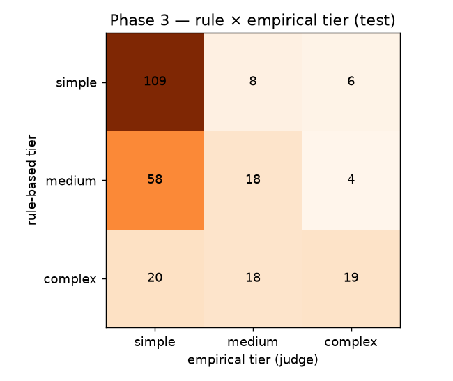
So what makes a case hard? The clue came from run 1 (report/fase3/analise_tier_empirico.md). The complexity label matched the tier that was actually needed in only 47.9% of messages. And a pattern showed up:
- messages without an order number: the cheap model passed 93.3% of them;
- messages with an order number: the cheap model passed only 22.7%.
What trips the cheap model is cross-checking order data against store policy. That finding is what motivated v2_ctx, which gets the tool output in its state. It was the best of the three, but not by enough to be significantly ahead of always-mid.
And c0541 shows the next level up: cross-checking isn’t always enough. Sometimes you have to notice that the customer is saying something the data contradicts.
What I can’t claim
- Labels haven’t been reviewed by a human. The templates were written with help from an LLM and the labels come from rules, not yet reviewed.
- Single judge. Only DeepSeek V4.1 Flash as LLM-as-judge, not yet calibrated against human ratings. Scores saturate at 4.75, which flattens differences. There may be a bias toward the expensive model’s longer replies.
- Synthetic data and mock tools. Scripted history, decision on the last message, no real tool-calling.
- The edge on complex cases is exploratory. 57 cases, analysis chosen after seeing the data.
- One location. Latency measured from a single Linux server in São Paulo.
- No generative router baseline. I didn’t compare against GPT-6 Luna as a router or against other decision models.
How to reproduce it
You need Python 3.11+. The harness is stdlib-only; the charts use matplotlib.
git clone https://github.com/gabrielcaiana/poc-modelos-de-decisao
cd poc-modelos-de-decisao
python3 -m venv .venv && .venv/bin/pip install matplotlib
cp .env.example .env   # OPENROUTER_API_KEY, export it in your shell

# tests and dry run, zero cost
python3 -m unittest -v tests.test_poc
python3 -m harness.fase3.run_grid --mock --split calib --limit 20 --out runs/mock-grid

# zero cost: reuse the recorded grid
python3 -m harness.fase3.replay runs/fase3-grid          # RESULTADOS_FASE3.md + replay_resultado.json
.venv/bin/python -m harness.fase3.figuras runs/fase3-grid
python3 -m harness.fase3.show runs/fase3-grid c0541     # trace of one conversation

# from scratch, real API
python3 datasets/fase3/gerar_conversas.py --n 1000
python3 -m harness.fase3.run_grid --live --split calib --session-cap 1 --out runs/fase3-grid
python3 -m harness.fase3.replay runs/fase3-grid --congelar   # calibration only: freezes τ1 and Layer 2
python3 -m harness.fase3.run_grid --live --split teste --session-cap 2 --out runs/fase3-grid
python3 -m harness.fase3.replay runs/fase3-grid
I re-ran the replay and the mock dry run to check these steps. The --session-cap values in the “from scratch” block are just a suggested per-run ceiling.
The cheapest way to check my numbers is the middle block: grid.jsonl is in the repo, and replay never calls the API.
What’s next
With the empirical oracle hitting 4.706 at mid-tier cost, the path forward is teaching Layer 2 to predict the empirical tier instead of the rule-based label. Before that: human review of the labels, calibrating the judge against a blind sheet, and a judge with more resolution.
If you have a chatbot in production, you can try this today: take a few hundred real, anonymized messages and run them all through your mid-tier and expensive models. Where does the mid-tier one lose? If the answer is “almost never,” you’ve got your decision. If it’s “the ones that cross order data with policy,” that’s where a decision model starts to earn its keep.
The code, logs and grid are at github.com/gabrielcaiana/poc-modelos-de-decisao.